NeurIPS 2026 Workshop · TAE (Trust‑AI‑Eval): Can We Trust AI Evaluation?
When Evaluation Goes Blind
Analyzing Patch‑Grid Failure Modes in Vision Transformers
Steffen Jung · Margret Keuper
University of Mannheim · Max Planck Institute for Informatics, Saarland Informatics Campus
Key finding
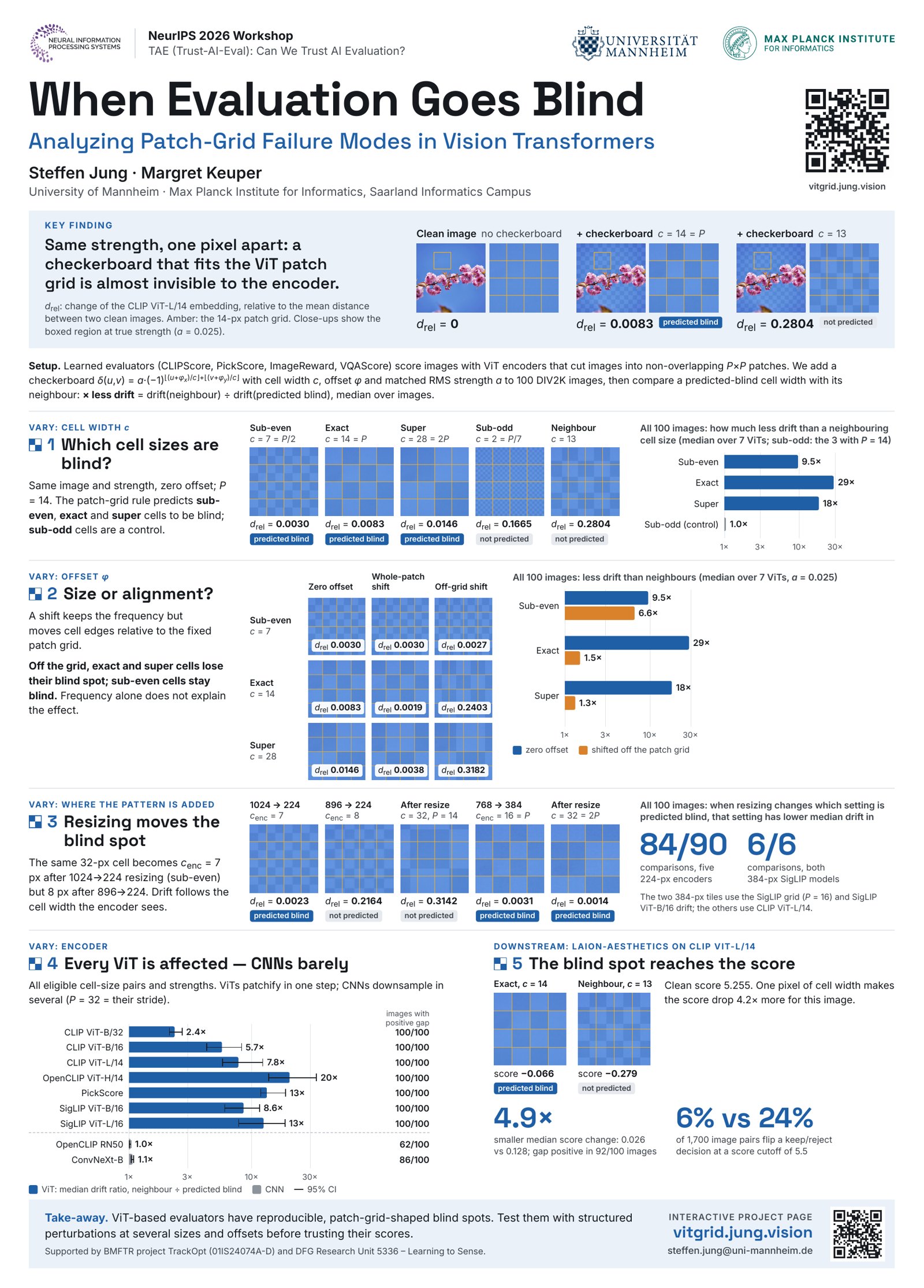
Same strength, one pixel apart: a checkerboard that fits the ViT patch grid is almost invisible to the encoder.
drel: change of the CLIP ViT‑L/14 embedding, relative to the mean distance between two clean images. Amber lines: the 14‑px patch grid. Close‑ups are contrast‑amplified ×8 for visibility; the full images show true strength (a = 0.025).
Clean image no checkerboard
drel = 0
+ checkerboard c = 14 = P
drel = 0.0083predicted blind
+ checkerboard c = 13
drel = 0.2804not predicted
Abstract
Can a learned evaluator miss a structured artifact?
Automated vision‑language evaluators rely on image encoders such as vision transformers (ViTs). We test whether the patch grid of a ViT reduces sensitivity to particular image changes. We overlay checkerboards with varying cell size, alignment, and preprocessing at controlled perturbation magnitude. Across seven ViTs, checkerboards at certain cell sizes cause smaller changes in encoder outputs than checkerboards at nearby sizes. Two convolutional controls show much weaker effects, while one aesthetic‑scoring model shows the same sensitivity difference. These findings reveal a reproducible evaluation blind spot: checkerboard perturbations applied at the same strength can produce sharply different responses depending on their scale and alignment relative to the model's patch grid.
Interactive
Try the probe yourself
Add a checkerboard δ(u,v) = a·(−1)⌊(u+φx)/c⌋+⌊(v+φy)/c⌋ to the paper's example image (DIV2K #0898) and see how it sits on the encoder's patch grid. Wherever the paper measured that exact setting, the panel shows the measured embedding change for this image and the median over all 100 images.
Encoder input with patch grid. Drag to move the close‑up box.
Close‑up: 4×4 patches
x
y
This image · drel—
Median over 100 images · drel—
The hypothesis
The patch‑grid rule
A ViT cuts its input into non‑overlapping P×P patches. Let cenc be the checker cell width at the encoder input. At zero offset, we predict reduced sensitivity in three cases, and use sub‑odd patterns as a control. Numbers below: how much less a predicted‑blind cell size moves the embedding than a neighbouring size (median over 7 ViTs, all 100 images, a = 0.025; sub‑odd: the 3 encoders with P = 14).
Interactive · full data
Every cell width from 1 to 112 pixels
Median relative drift across the 100 images when the checkerboard is added after resizing at zero offset. Filled blue points satisfy the patch‑grid rule; the drops line up with them. Hover for values, click a point to load it into the playground above.
Median image‑level blindness gap Δblind = log10 d(neighbour) − log10 d(predicted blind). CNNs use their output stride 32 as P.
ViTCNN— 95% image‑bootstrap CI (combined only)
Show as table
2 · Size or alignment?
Shifting a checkerboard keeps its frequency but moves cell edges relative to the fixed patch grid. Off the grid, exact and super cells lose most of their blind spot; sub‑even cells stay blind. Frequency alone does not explain the effect.
zero offsetshifted off the patch grid
3 · Resizing moves the blind spot
The same 32‑px source cell becomes 7 px after 1024→224 resizing (two cells per 14‑px patch: sub‑even) but 8 px after 896→224 (no rule). Drift follows the cell width the encoder actually sees. When resizing changes which setting is predicted blind, that setting has lower median drift in:
84/90comparisons, five 224‑px encoders
6/6comparisons, both 384‑px SigLIP models
Try it: in the playground, pick CLIP ViT‑L/14, set c = 32 and switch between “1024 px source” and “896 px source”.
4 · The blind spot reaches a downstream score
The public LAION‑Aesthetics predictor on CLIP ViT‑L/14 embeddings inherits the effect. At a = 0.025, the median absolute score change is 0.026 for predicted‑blind patterns versus 0.128 for neighbouring patterns, and the score‑space gap is positive for 92 of 100 images.
4.9×smaller median score change
0.62log₁₀ score‑space gap
For the example image (clean score 5.2551), the exact c = 14 pattern lowers the score by 0.0661; its c = 13 neighbour lowers it by 0.2794 — about 4.2× more.
Keep/reject decisions flipped by the checkerboard
A filter keeps images scoring at or above the cutoff. Out of 1,700 matched condition–image pairs:
From the paper
Figures
Click to enlarge.
Poster
Workshop poster
The poster walks through the same five questions — which cell sizes are blind, size versus alignment, resizing, encoder families, and the downstream score — using close‑ups of the example image at true perturbation strength.
ViT‑based evaluators have reproducible, patch‑grid‑shaped blind spots. Test evaluators with structured perturbations at several sizes and spatial offsets before relying on their scores for benchmarking, filtering, or model comparison.
Code
Probe your own evaluator
The probe itself is a few lines of code: add the checkerboard after the encoder's resize/crop and before channel normalization, then compare embedding drift for a predicted‑blind width against its neighbours.
import numpy as np
def checkerboard(h, w, c, a, phi=(0, 0)):
"""delta(u,v) = a * (-1)^(floor((u+phi_x)/c) + floor((v+phi_y)/c)), same for all RGB channels."""
u = np.arange(w)[None, :] + phi[0]
v = np.arange(h)[:, None] + phi[1]
return a * (-1.0) ** ((u // c) + (v // c))
def perturb(x, c, a, phi=(0, 0)):
"""x: H x W x 3 image in [0,1] at the encoder input (after resize/crop, before normalization)."""
d = checkerboard(x.shape[0], x.shape[1], c, a, phi)[..., None]
return np.clip(x + d, 0.0, 1.0)
def rel_drift(z, z_pert, D_f):
"""z, z_pert: unit-L2 embeddings; D_f: mean cosine distance between clean images."""
return (1.0 - (z * z_pert).sum(-1)) / D_f
def blindness_gap(d_neighbour, d_blind):
"""Positive = smaller response to the predicted-blind width; 1.0 = tenfold lower drift."""
return np.log10(d_neighbour) - np.log10(d_blind)
# e.g. a ViT with P = 14: compare c = 14 (exact) with c = 13 and c = 15 at a = 0.025
Citation
BibTeX
@inproceedings{jung2026blind,
title = {When Evaluation Goes Blind: Analyzing Patch-Grid Failure Modes in Vision Transformers},
author = {Jung, Steffen and Keuper, Margret},
booktitle = {NeurIPS 2026 Workshop on Trust-AI-Eval (TAE): Can We Trust AI Evaluation?},
year = {2026},
url = {https://openreview.net/forum?id=sZ1Du9f3GA}
}